Is the 4% Rule Still Safe?
Real history and textbook Monte Carlo agree the 4% rule works below 4.5% and disagree above it. No historical retirement started this expensive.
Every retirement calculator answers this with Monte Carlo: fit a mean and a volatility to stock and bond returns, draw random numbers, see how often the money runs out. I built three versions of that test — real historical retirements, a textbook Monte Carlo, and a fairer resampling method — expecting real history to look the most dangerous, because actual markets have fatter tails than a bell curve assumes.
That is not what happened. Below a 4.5% withdrawal rate, real history is the safest of the three methods. Above it, real history is the most dangerous. And there is a fact buried in the valuation data that matters more than either result: not one of the 840 real 30-year retirements in this test ever started as expensive as today’s market.
The three ways to ask the question
Real history. Every actual rolling 30-year retirement start in the US stock/bond record — not a simulation, but what would actually have happened to someone who retired in each of 840 different months. This is the method behind the original 4% rule.
Normal Monte Carlo. The textbook approach, and what most calculators actually run: fit a mean and covariance to the same historical data, draw independent normal monthly returns, assume a fixed inflation rate. Ten thousand simulated 30-year paths.
Block-bootstrap Monte Carlo. A fairer simulation. Instead of fitting a bell curve, it resamples real historical 24-month blocks of stock, bond and inflation data together, with replacement, and stitches them into 30-year paths. This keeps the real fat tails and the real relationship between stocks, bonds and inflation, while scrambling the order events happened in. Also ten thousand paths.
All three run on the same underlying series: the same validated 60/40 portfolio I built for the 60/40-is-dead post — Ken French US market returns and a constant-maturity 10-year Treasury total return constructed from month-end yields, 1926 to 2026. A retiree withdraws 4% of the starting balance, then that same real (inflation-adjusted) dollar amount every year for 30 years, rebalanced annually.
Real history looked safer than Monte Carlo — until it didn’t
| Method | Failure rate at a 4% withdrawal rate |
|---|---|
| Real history (840 actual retirements) | 5.1% |
| Normal Monte Carlo (textbook) | 6.8% |
| Block-bootstrap Monte Carlo | 8.9% |
If the story were simply “fat tails make reality more dangerous than a bell curve,” real history would be the worst number here. It is the best. But push the withdrawal rate up and the ranking flips completely:
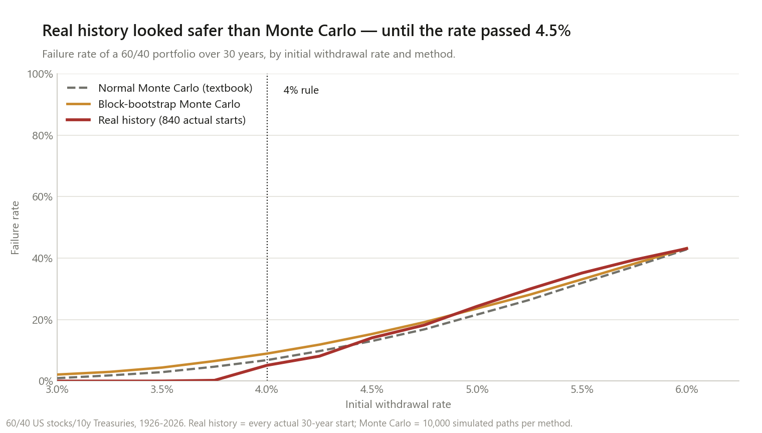
| Withdrawal rate | Real history | Block-bootstrap MC | Normal MC |
|---|---|---|---|
| 3.00% | 0.0% | 2.1% | 0.9% |
| 3.75% | 0.2% | 6.5% | 4.7% |
| 4.00% | 5.1% | 8.9% | 6.8% |
| 4.50% | 14.0% | 15.3% | 13.0% |
| 5.00% | 24.3% | 23.6% | 21.6% |
| 6.00% | 43.1% | 43.2% | 42.8% |
By 6%, all three methods agree almost exactly. The disagreement is concentrated precisely in the range anyone actually uses.
Where the real failures actually came from
Every single one of the 43 failing starts — 5.1% of 840 — began between August 1964 and June 1969. Not scattered across the sample. One five-year window. A retiree who started in February 1966 ran out of money in year 26 of 30; one who started in July 1967 ran out in year 28. Every other decade in the 100-year sample produced zero failures at a 4% rate. A follow-up post isolates exactly why 1966 failed: reshuffle that retiree’s own 30 annual returns into a different order and 96.5% of the reshuffles survive. It was not the amount the market returned. It was the order it arrived in.
That is the whole explanation for the crossover. A hundred years of monthly data produces 840 overlapping 30-year windows, but a 30-year window only fits into a 100-year sample about 1199 ÷ 360 ≈ 3.3 times without overlapping itself. Real history is not 840 independent tests of the 4% rule. It is closer to three or four, viewed through a sliding window that makes them look like hundreds.
Monte Carlo does not have that problem — it draws 10,000 genuinely independent 30-year sequences — so at low withdrawal rates it keeps finding bad-luck combinations that this particular 100 years of market history simply never produced. That is what “normal Monte Carlo says 6.8%, real history says 5.1%” actually means: not that Monte Carlo is too pessimistic, but that a single realized century is a small sample, and this test asks it a low-probability question.
The crossover above 4.5% is the flip side of the same fact. Once the failure threshold gets low enough that more than just the 1966 cohort starts failing, real history’s failures arrive in the same clusters its successes did — concentrated, lumpy, all-at-once — while Monte Carlo’s stay smooth. The lumpiness is what a small independent sample looks like next to a large one, in both directions.
What each method would call “safe”
Two different bars produce two different pictures. First, the rate at which failures hit literally zero — a very strict bar for Monte Carlo, since it is asking that not one of 10,000 independent draws fail:
| Method | 0% failures | Failure rate ≤ 5% (“95% confidence”) |
|---|---|---|
| Real history | 3.70% | 4.00% |
| Normal Monte Carlo | 1.60% | 3.80% |
| Block-bootstrap Monte Carlo | 1.15% | 3.60% |
At the conventional 95%-confidence bar that most retirement research actually uses, the three methods land within 40 basis points of each other — real history is if anything the most generous. But demand that a method has never once failed, and the picture splits wide open: real history’s “never failed” rate is 3.70% simply because it has only ever run the experiment three or four independent times. Monte Carlo, running it 10,000 times, finds a genuine failure somewhere above 1.15–1.60% and keeps that verdict.
Neither number is wrong. They are answers to different questions: “did this ever fail in the history we happen to have” versus “how often would this fail across the wider space of sequences that history could plausibly have produced instead.”
The valuation nobody’s safe rate was tested against
Here is the fact that made me stop treating the historical 3.70–4.00% range as reassuring.
| Starting CAPE (cyclically-adjusted P/E) | |
|---|---|
| Median across all 840 historical starts | 14.7 |
| The failing 1964–69 cohort | 17.3 – 24.1 |
| Most recent available (September 2024) | 35.2 |
Splitting the 840 starts at the median CAPE makes the pattern explicit: retirements that began below the median starting valuation had a 0.0% failure rate. Above the median, 10.2%. Every one of the 43 failures came from a start with above-median CAPE — the 1966 cohort’s valuation, in the high teens to low twenties, was already on the expensive side of history.
Today’s CAPE is not on the expensive side. It is higher than all 840 of the historical starting points this whole test is built from — the 97th percentile of the full CAPE record back to 1881. The only period that ever ran higher was the dot-com peak around 1999–2000, and that cohort has not finished a 30-year test yet; the data this post uses ends mid-2026. A later post traces that cohort’s actual account balance, year by year, against the one that failed — so far, a very different outcome.
I want to be precise about what this does and does not say. It is not a forecast — this site does not make those, and CAPE is a notoriously poor short-term timing tool. A later post tests exactly how poor: real long-horizon predictive power, and an out-of-sample forecast that goes sharply negative the moment a CAPE-fitted line has to generalise past the data it was trained on — which is exactly the position today’s reading puts it in. It is a narrower, checkable statement: the historical failure rate of 3.7–5.1% was earned entirely by cohorts starting at valuations between roughly 9 and 24. Nobody in the sample has tested what happens starting from 35. The 4% rule’s historical safety record is real, and it has never been tested under today’s starting condition.
Does the asset mix change the answer?
| Stocks / bonds | Real history failure rate | Normal MC failure rate |
|---|---|---|
| 40 / 60 | 10.0% | 6.6% |
| 50 / 50 | 7.0% | 6.5% |
| 60 / 40 | 5.1% | 6.8% |
| 70 / 30 | 4.4% | 7.2% |
| 80 / 20 | 3.5% | 8.1% |
This is a smaller finding, but an unexpected one: the two methods do not just disagree on magnitude, they disagree on direction. Real history says more stocks made every allocation tested safer, all the way to 80/20 — the realized US equity premium was large enough to outrun a fixed real withdrawal. Normal Monte Carlo says the opposite: more stocks means more volatility means more failures, because a symmetric bell curve cannot represent the fact that stocks’ real-world returns compound better than their volatility alone would suggest. Which one you believe changes whether the “safe” move is more stocks or fewer.
What this does and doesn’t change
It does not mean the 4% rule is broken. At a conventional 95% confidence bar, all three methods — real history included — support a rate close to 4%, not a collapse to 2% or 3%.
It does mean the “96 years of history back it up” comfort is thinner than it sounds. Ninety-six years of monthly data is not ninety-six independent tests. It is roughly three. One of those three happened to contain a bad cohort; the other two did not. That is a small sample behaving exactly like a small sample, not evidence of robustness.
It does mean the valuation question is the live one. Not “is 4% safe on average,” which this data answers reassuringly, but “has 4% ever been tested starting from here” — which it has not.
It does mean these failure rates are a floor, not a ceiling. Every number on this page is fee-free. A follow-up post quantifies what a real fee does to them: a 1% advisor fee alone nearly triples the historical failure rate, from 5.1% to 13.7%.
Method notes and limitations
- Annual withdrawals and rebalancing. The classic Bengen convention: withdraw a fixed real dollar amount once a year, rebalance to target weights right after. Monthly withdrawals or rebalancing would change the numbers slightly, probably in the direction of fewer failures (smoother cash-flow timing).
- The 840 “windows” are not 840 independent trials. Stated above, worth restating: they overlap so heavily that the sample contains only about three independent 30-year eras. Treat the real-history failure rate as a description of one realized century, not as a large-sample statistical estimate.
- Normal Monte Carlo uses historical mean/covariance and a fixed inflation rate — the historical average, applied every year. A calculator using lower forward-looking return assumptions (common practice given current valuations) would show higher failure rates across the board than what is reported here.
- Block-bootstrap uses 24-month blocks. Long enough to preserve most of a recession or a rate cycle inside one block, short enough to build many distinct 30-year paths. A different block length would shift the bootstrap numbers modestly.
- US-only, two assets. Stocks are the Ken French US market; bonds are a constructed constant-maturity 10-year Treasury, validated against IEF at r = 0.990. No international diversification, which earlier posts on this site found adds less than it looks like it should.
- No fees, no taxes, no Social Security, no spending flexibility. A real retiree who cuts spending after a bad decade fails less often than this model allows.
- CAPE data runs through September 2024 (Shiller’s published series); the stock, bond and inflation series run through June 2026. The valuation comparison uses the last available CAPE reading, about two years stale relative to the return data.
- Fixed 30-year horizon. A shorter retirement fails less often at any given rate; a longer one fails more.
This is research, not personalised financial advice.
The code
The engine simulates every path — real or simulated — the same way:
def simulate(stock_r, bond_r, infl_r, weight_stock, swr, months=360):
    """Vectorized withdrawal simulation across N paths at once.

    stock_r, bond_r, infl_r: (N, months) monthly nominal returns / inflation.
    Withdraw swr * balance0 at the START of each year, escalated by realised
    inflation since year 0 -- the actual Bengen rule: a fixed REAL dollar
    amount, not a fixed percentage of the current balance.
    """
    n = stock_r.shape[0]
    balance, cum_infl = np.ones(n), np.ones(n)
    alive = np.ones(n, dtype=bool)
    for yr in range(months // 12):
        balance = balance - swr * cum_infl
        alive &= balance > 0
        bal = np.where(alive, balance, 0.0)
        s_bal, b_bal = bal * weight_stock, bal * (1.0 - weight_stock)
        for m in range(12):
            i = yr * 12 + m
            s_bal *= (1.0 + stock_r[:, i])
            b_bal *= (1.0 + bond_r[:, i])
            cum_infl *= (1.0 + infl_r[:, i])
        balance = s_bal + b_bal
    return {"survived": alive, "failure_rate": 1.0 - alive.mean()}


def block_bootstrap(stocks, bonds, infl, n_sims, months=360, block=24, seed=0):
    """Resample real (stock, bond, inflation) blocks together, with replacement.

    Keeps the real joint distribution and its fat tails; scrambles the order
    blocks are stitched into a 30-year path.
    """
    rng = np.random.default_rng(seed)
    sv, bv, iv = stocks.to_numpy(), bonds.to_numpy(), infl.to_numpy()
    T, n_blocks = len(sv), -(-months // block)
    S = np.empty((n_sims, n_blocks * block)); B, I = np.empty_like(S), np.empty_like(S)
    for k in range(n_blocks):
        starts = rng.integers(0, T - block, size=n_sims)
        idx = starts[:, None] + np.arange(block)[None, :]
        S[:, k*block:(k+1)*block] = sv[idx]
        B[:, k*block:(k+1)*block] = bv[idx]
        I[:, k*block:(k+1)*block] = iv[idx]
    return S[:, :months], B[:, :months], I[:, :months]
Data: Ken French US market total return (1926– ), a 10-year Treasury total return constructed from month-end yields (Shiller pre-1962, FRED DGS10 after), FRED CPI, and Shiller’s cyclically-adjusted P/E, all validated the same way as the 60/40 post that shares this dataset.
The code is above in full. If you re-run it and the crossover lands somewhere other than 4.5%, I want to know why.