Sequence of Returns Risk, Quantified
Reshuffle the exact same 30 years of returns 10,000 times. A lump sum never notices. A retiree fails or thrives by it. A saver benefits from the reverse.
The last post found that a retiree who started in 1966 ran out of money, while almost every other 30-year period in the historical record was fine. The natural next question is whether 1966 was a bad 30 years or a bad order — whether the market simply returned too little, or whether the same return arrived in an arrangement that happened to be lethal for someone withdrawing from it.
This isolates the answer directly. Take the actual 30 annual returns from 1966–1995 — the exact same 30 numbers, nothing simulated — and shuffle their order thousands of times. Every shuffle compounds to the identical 30-year return, by construction. Whatever difference shows up in the outcome cannot be about how much the market returned. It can only be about when.
The control case: a lump sum cannot have this problem
Before touching withdrawals, it is worth proving that sequence risk is not a property of returns at all — it is a property of cash flows interacting with returns. A lump sum, rebalanced annually with nothing added or removed, turns 30 annual returns into a straight multiplication: final value equals the product of each year’s growth factor. Multiplication does not care what order you do it in.
| Era | 30-year lump-sum multiple | Across 10,000 reshuffles of its own returns |
|---|---|---|
| 1929–1958 | 7.7777× | min 7.7777× — max 7.7777× |
| 1966–1995 | 16.6497× | min 16.6497× — max 16.6497× |
| 1996–2025 | 10.8523× | min 10.8523× — max 10.8523× |
Ten thousand random reorderings, four decimal places, zero variance. This is not a
near-result — it is the algebraic identity a×b×c = c×a×b showing up in financial data.
It matters because it pins down exactly what ingredient is required for sequence to matter
at all: a cash flow. Nothing else about a portfolio’s mechanics creates this risk.
Add a withdrawal, and order stops being irrelevant
Same 1966–1995 returns, same 10,000 reshuffles, now with the 4% withdrawal rule from the last post running against each one.
| Real historical order | Across 10,000 reshuffles of the same returns | |
|---|---|---|
| 1929–1958 | Survived | 8.4% fail |
| 1966–1995 | Failed, year 26 | 3.5% fail |
| 1996–2025 | Survived | 0.0% fail (1 of 10,000) |
The actual 1966 retiree landed in roughly the worst 3.5% of every way these exact 30 years could have been arranged. Reorder the identical returns and 96.5% of the time the money lasts the full 30 years. The 30-year return was never the problem — a 16.65× lump-sum multiple over 30 years is a perfectly good outcome. The problem was drawing one of the unlucky orderings out of a set where the vast majority were fine.
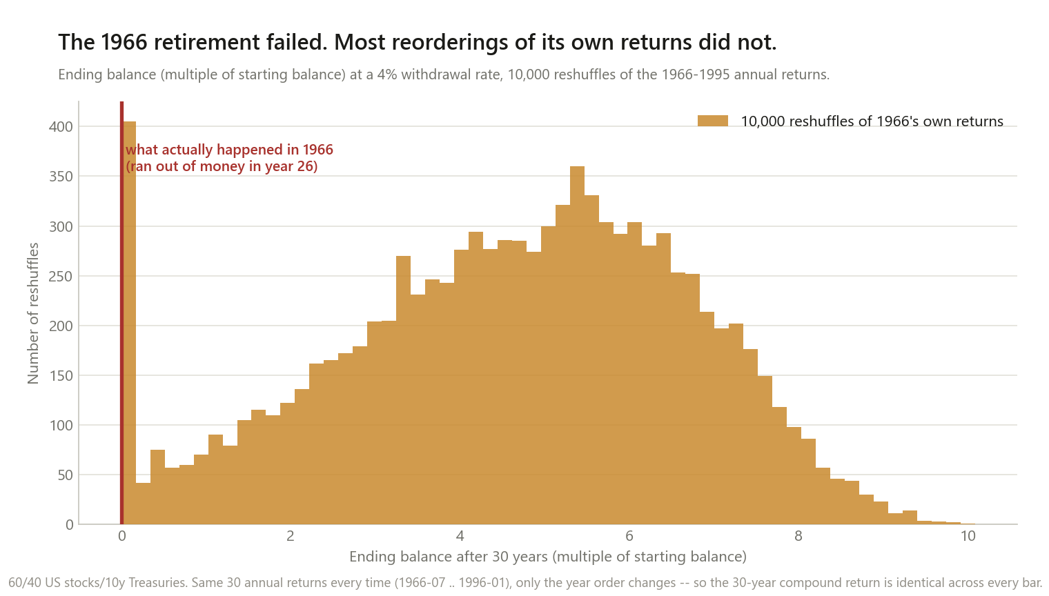
1929 cuts the other way: it actually survived, but 8.4% of its own possible reorderings would have failed it — a smaller, calmer-looking 30-year return (7.78× vs 16.65×) that turned out to be more dangerous to reshuffle, because more of its bad years cluster together no matter how you arrange them.
Add a contribution instead, and the effect flips
Withdrawing is not the only cash flow that interacts with sequence. Contributing does too — dollar-cost averaging into the market, the ordinary saving that happens for the 30-plus years before retirement. Same reshuffled returns, same 30 years, but now a fixed real amount goes in every year instead of coming out.
| Era | Ending balance across 10,000 reshuffles (p10 – median – p90) | Spread |
|---|---|---|
| 1929–1958 | 51.7 – 75.7 – 111.0 | 2.1× |
| 1966–1995 | 48.5 – 61.0 – 77.7 | 1.6× |
| 1996–2025 | 66.4 – 77.7 – 92.8 | 1.4× |
The spread is real, but it is the correlation that makes the mechanism visible. Across all three eras, a worse first-decade return predicted a better ending balance for a saver — strongly: −0.73, −0.79, −0.83. That is the buying-the-dip mechanism running in reverse of the withdrawal case. A retiree hit by bad returns early is drawing down a shrinking pile at the worst possible time. A saver hit by bad returns early is buying more of the market cheap, for decades, before the eventual recovery. Same reshuffled returns, same 60/40 portfolio, opposite sign.
Which part of the sequence actually matters
Isolating the first decade specifically, within the 1966 reshuffles:
| First-decade return (of that reshuffle) | Withdrawal failure rate |
|---|---|
| Best 10% of reshuffles (+264% or better over 10 years) | 0.0% |
| Worst 10% of reshuffles (+80% or worse over 10 years) | 27.4% |
Notice that even the “worst” first decade here is not a crash — +80% over ten years is about 6.1% a year, a perfectly respectable run. It is still worse, by the standards of what this specific 30 years could produce, and that alone is enough to move the failure rate from zero to better than one-in-four. You do not need a crash in the first decade to create sequence risk. You just need the first decade to land in the worse half of what was available.
One honest complication: the last decade’s return correlates negatively with survival in this data (−0.33 to −0.48 across the three eras), which looks backwards at first glance. It is not an independent finding — it is an arithmetic echo of the first-decade effect. Because the 30-year total return is fixed, an unusually strong first decade mechanically leaves less return available for the remaining twenty years to distribute, which pulls the last decade down along with it (the two are correlated at −0.44 to −0.49 across shuffles). Do not read this as “bad returns late in retirement help” — read it as a reminder that partitioning one fixed total into pieces creates statistical relationships between the pieces that have nothing to do with cause and effect.
This is not one anecdote — it holds across all 840 real windows
Every one of post 12’s 840 real historical 30-year starts got the same treatment: reshuffle its own 30 annual returns a few hundred times, and see how often the real historical outcome would have gone the other way.
| Result | |
|---|---|
| Windows that really survived, but ≥10% of their own reshuffles fail | 52 of 797 (6.5%) |
| Windows that really failed, but ≥50% of their own reshuffles survive | 43 of 43 (100%) |
| Median shuffle-failure-rate across all 840 windows | 0.7% |
| Real historical failure rate (from post 12) | 5.1% |
That middle row is the whole post in one number. Every single historical failure of the 4% rule — the entire 1964–69 cohort — would have mostly survived had its own 30 years of returns simply arrived in a different order. None of them were doomed by the amount the market returned over their 30 years. All of them were unlucky in when.
What this does and doesn’t change
It does not mean sequence risk is rare. The 1964–69 cohort was not a freak one-in-a-million draw — it landed in the worst 3.5% of its own possible orderings, and nine other historical windows separately produce a failure at a 4% rate. A 3–7% chance of an unlucky ordering is a real, recurring feature of retirement planning, not an edge case to dismiss.
It does mean “the market only returned X% over your 30 years” is the wrong autopsy for a failed retirement. The right question is not how much return arrived, but when. A 16.65× lump-sum multiple failed a withdrawer and comfortably succeeded for a saver, using the identical returns.
It does mean withdrawal order and contribution order are mirror-image risks, not the same risk. A strategy that reduces one (holding more in cash early, for instance) does not automatically reduce the other, because they are hurt by opposite orderings of the same returns.
This site does not turn findings like this into a specific rule for what to do about it — that is a personal decision that depends on flexibility, other income, and risk tolerance none of this data can see. What it can say is narrower and checkable: the risk this post measures is about order, not magnitude, and it is large enough to turn a certain failure into a 96.5% success rate without changing a single one of the 30 numbers involved.
It does mean the first decade specifically is where to look next. A later post checks that directly against the real, un-reshuffled record — every historical failure of the 4% rule came from the worst fifth of real first-decade returns — and traces two real cohorts with a bad first decade, 1966 and 2000, to see how far the resemblance actually goes.
Method notes and limitations
- Shuffled by whole year, not by month. Each 12-month block moves as a unit, preserving the real within-year pattern (a crash and its recovery inside one year stay together) while randomising the order years occur in. Shuffling at the monthly level instead would show a similar effect, diluted, since it breaks up real short-term return clusters that a whole-year shuffle keeps intact.
- This is not the same operation as post 12’s block-bootstrap. That resampled with replacement from the full 100-year pool, building new combinations that never historically happened. This reshuffles without replacement — always the same 30 numbers from one real 30-year stretch, so the compound return is identical across every permutation by construction, not just similar.
- The last-decade correlation is confounded, as described above — a mechanical byproduct of partitioning a fixed total, not independent evidence about late-retirement timing. Reported for transparency, not as a finding to act on.
- 10,000 reshuffles per era, 400 per window in the 840-window robustness check — enough to estimate failure rates to within roughly a percentage point at this sample size, not enough to resolve differences much finer than that.
- Three illustrative eras, chosen for spread and for the direct link to post 12 (1966 is the exact failing cohort from that post), not a random or exhaustive sample of eras.
- 60/40, annual rebalancing, 4% withdrawal or $1 real contribution per year — the same conventions as post 12, for direct comparability.
- No fees, taxes, Social Security, or spending flexibility, as in post 12.
This is research, not personalised financial advice.
The code
The reordering trick, and the proof that it leaves the compound return untouched:
def random_perms(n_shuffles, years, seed):
    rng = np.random.default_rng(seed)
    return np.argsort(rng.random((n_shuffles, years)), axis=1)


def apply_perm(arr_1d, perms, block=12):
    """Reorder whole 12-month year-blocks of arr_1d according to `perms`.

    arr_1d: length years*block, ONE fixed real sequence. perms: (n_shuffles,
    years), each row a permutation of 0..years-1. Every output row contains
    the same 12*years numbers, only reordered by year -- so every row
    compounds to the identical total return.
    """
    years = len(arr_1d) // block
    A = arr_1d.reshape(years, block)
    return A[perms].reshape(perms.shape[0], years * block)


# same 1966-1995 returns, 10,000 different orders
perms = random_perms(10_000, 30, seed=20260828)
S_sh = apply_perm(stock_r, perms)
B_sh = apply_perm(bond_r, perms)
I_sh = apply_perm(infl_r, perms)

lump  = simulate(S_sh, B_sh, I_sh, 0.60, swr=0.0)    # -> zero variance
withdr = simulate(S_sh, B_sh, I_sh, 0.60, swr=0.04)   # -> 3.5% fail
simulate() is the same withdrawal engine from the 4% rule
post, now shared in one module so both posts run
identical accounting. Data: the same Ken French / constructed-Treasury / FRED CPI series
validated in the 60/40 post.
Reorder your own 30 years and get a different failure rate than 3.5%? That would mean my random seed is doing more work than it should be — tell me.