Does Low-Volatility Investing Actually Work?
In a no-lookahead backtest, high-volatility stocks won on raw return and low-volatility stocks won on drawdown. Sharpe ratios were nearly identical.
The “low-volatility anomaly” is a specific, strong claim: stocks with lower historical volatility have gone on to deliver better risk-adjusted returns than volatile stocks, which shouldn’t happen if risk and return trade off the way finance textbooks say they do. The whitepapers making this claim mostly reach back 90 years and mostly stop well before now. This runs the actual test — rank real S&P 500 stocks by trailing volatility only, rebalance annually, hold forward, no lookahead anywhere — over the period an investor alive today would actually have lived through, then checks whether the real ETF built on this idea delivered it.
A genuine no-lookahead backtest, not a full-sample sort
The diversification post already built the infrastructure for this: today’s S&P 500 constituents, real monthly returns, same disclosed survivorship bias (companies that failed and dropped out of the index are missing, which flatters this test rather than helping the conclusion below). This adds a rule with a clock: each year, rank every stock by its trailing 12-month volatility — data that would actually have been available at the time — split into a low-volatility and a high-volatility quintile, hold both equally-weighted for the next 12 months, then re-rank.
| Portfolio | Annualised return | Volatility | Sharpe | Max drawdown |
|---|---|---|---|---|
| Low-volatility quintile | 11.16% | 12.42% | 0.90 | −38.2% |
| High-volatility quintile | 21.09% | 22.81% | 0.92 | −52.3% |
| Equal-weight benchmark (all stocks) | 14.71% | 16.10% | 0.91 | −46.7% |
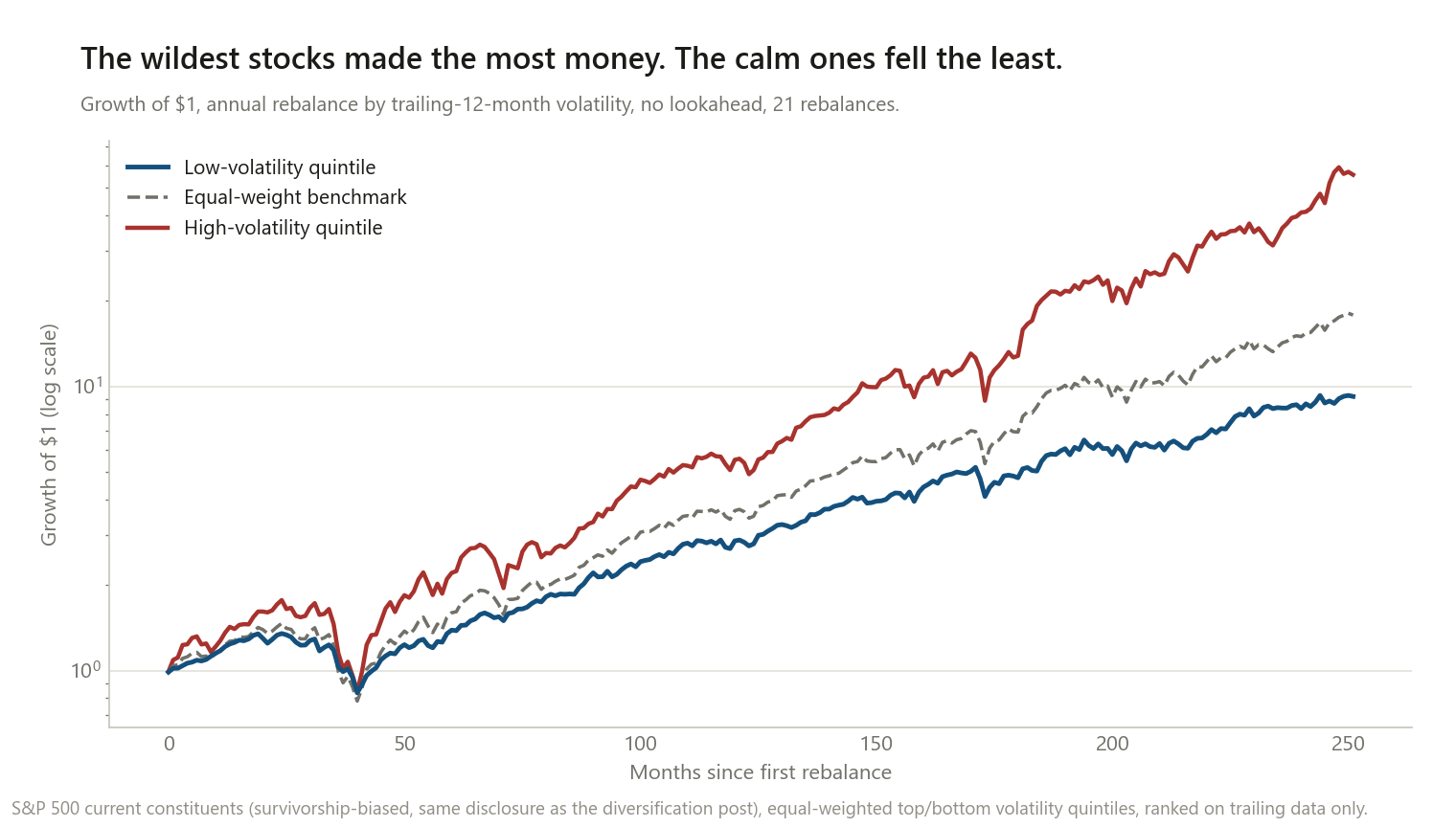
This is not the story the whitepapers tell. In this test, over this period, the high-volatility quintile won decisively on raw return — nearly double the low-volatility quintile’s number. What the low-volatility quintile actually delivered was a real, measurable reduction in maximum drawdown, not a higher return for the risk taken.
Sharpe ratios: this is where the “anomaly” claim actually lives, and it’s thin here
The specific claim isn’t “low-vol makes more money” — it’s “low-vol makes more money per unit of risk.” The Sharpe ratios above are 0.90, 0.92, and 0.91: essentially indistinguishable. Formally testing the low-volatility quintile’s return against its own (lower) market exposure:
| Value | |
|---|---|
| Low-vol beta to the benchmark | +0.69 |
| Alpha after adjusting for that beta (annualised) | +1.03% |
| t-statistic | 0.82 |
There’s a positive point estimate — low-volatility stocks delivered slightly more return than their reduced market exposure alone would predict — but a t-stat of 0.82 is far from conventional significance. In this specific test, on this specific universe and period, the low-volatility anomaly is a hint, not a finding.
The real, buyable version: USMV against the market it’s supposed to beat
| USMV (min-vol) | SPY | |
|---|---|---|
| Annualised return (2011–2026, 177 months) | 11.76% | 15.11% |
| Volatility | 11.14% | 13.93% |
| Max drawdown | −19.1% | −23.9% |
| Alpha vs. SPY (annualised) | +1.39% | — |
| t-statistic on that alpha | 0.94 | — |
The real fund tells the same story as the backtest, more starkly. USMV has trailed SPY by 3.35 percentage points a year in raw terms since its 2011 launch — a period dominated by a small number of very large, very volatile technology stocks that a low-volatility screen structurally underweights. What USMV did deliver, reliably: meaningfully lower volatility (11.14% vs. 13.93%) and a shallower max drawdown (−19.1% vs. −23.9%). The risk-adjusted alpha is again positive (+1.39%/yr) and again not statistically significant (t=0.94) over this sample length.
What this does and doesn’t change
It does not mean low-volatility investing “worked” in the sense most marketing for it implies. Neither the backtest nor the real fund showed low-vol beating the market on raw return, and the risk-adjusted edge in both cases was positive but not statistically convincing.
It does mean low-volatility investing reliably does the one thing its name promises. Lower realised volatility and shallower drawdowns showed up in both the backtest and the live fund, consistently, which is a real and checkable claim even without a proven return premium attached to it.
It does mean this is a period-dependent story. A 2004–2026 (or 2011–2026) test sits inside a stretch dominated by a handful of enormous, volatile winners — the same return-skew mechanism already documented for individual stocks. A low-volatility screen is, almost by construction, going to underweight exactly the stocks driving that skew. Whether that’s a permanent feature of markets or a feature of this particular 20-year stretch isn’t something this test can resolve.
It does mean “smoother, not necessarily richer” is the honest pitch. If the reason to hold a low-volatility fund is the ride, not a proven excess return, that’s a coherent reason — it just isn’t the reason usually given.
Method notes and limitations
- Survivorship bias, same disclosure as the diversification post: today’s S&P 500 members only, so failed companies are missing entirely, which biases toward making low-volatility (the survivors, definitionally less prone to catastrophic single-stock blowups) look worse relative to a fairer test, not better — this test’s already-modest results are if anything flattered against that bias, not helped by it.
- Annual rebalance, quintile sort, equal-weighted within each quintile. A different rebalancing frequency, number of buckets, or weighting scheme would produce different numbers.
- Trailing 12-month volatility only as the ranking signal — the whitepapers behind the original anomaly research often use longer or differently-constructed volatility measures (some use idiosyncratic, beta-adjusted volatility rather than total volatility); a different construction could show a different result.
- 384 stocks with complete 21-year histories, out of 503 current constituents — the same complete-history filter the diversification post uses.
- USMV is one fund, one time period. 177 months is a short sample for resolving a modest effect at conventional statistical significance.
- Newey-West standard errors, 6 lags, matching the convention used across the momentum and small-cap posts.
This is research, not personalised financial advice.
The code
The no-lookahead ranking-and-holding loop — the part that makes this a backtest rather than a full-sample sort:
n_years = n_months // 12 - 1
for yr in range(n_years):
    form_start, form_end = yr * 12, yr * 12 + 12      # trailing 12m, used ONLY to rank
    hold_start, hold_end = form_end, form_end + 12      # next 12m, actually held

    trailing_vol = Rv[form_start:form_end].std(axis=0)  # known at the time
    order = np.argsort(trailing_vol)
    low_idx, high_idx = order[:QUINTILE], order[-QUINTILE:]

    hold = Rv[hold_start:hold_end]                       # returns NOT used in the ranking
    low_rets.append(hold[:, low_idx].mean(axis=1))
    high_rets.append(hold[:, high_idx].mean(axis=1))
The ranking window and the holding window never overlap. Nothing about how a stock performed during the period it’s held influenced which quintile it was placed in.
Data: same S&P 500 constituent list and yfinance monthly-return pipeline as the diversification post, plus real USMV and SPY monthly prices since USMV’s 2011 launch.
If a longer sample, a different volatility construction, or a different rebalancing rule pushes either alpha t-stat comfortably past 2, I want to know — that’s the specific bar this post couldn’t clear.