Do Dividend Stocks Actually Outperform?
High-yield stocks did beat low-yield stocks. But the entire advantage vanishes once you control for value, and here is the regression that shows it.
The case for dividend investing usually arrives as a chart: high-dividend stocks against the S&P 500, high-dividend wins, therefore buy dividend stocks.
I ran it on the full CRSP universe back to 1927, and the chart is right. High-yield stocks really did beat low-yield stocks.
Then I ran the step the chart never includes, and the result reversed.
The raw claim checks out
US stocks sorted into dividend-yield buckets each June, value-weighted, held for a year. Ken French’s data, 1927–2026, 1,188 months:
| Portfolio | Return/yr | Volatility | Sharpe | Worst drawdown |
|---|---|---|---|---|
| Top 30% by dividend yield | 11.32% | 19.58% | 0.48 | −87.9% |
| Middle 40% | 10.68% | 17.64% | 0.48 | −85.5% |
| Bottom 30% (lowest payers) | 10.10% | 19.47% | 0.43 | −81.3% |
| Pays no dividend at all | 9.47% | 28.05% | 0.35 | −90.3% |
| The whole market | 10.37% | 18.34% | 0.45 | −83.7% |
High yield beat low yield by 1.22 percentage points a year for ninety-nine years. Over that span, compounded, that is an enormous difference in ending wealth. The dividend advocates are not making the number up.
Notice the first crack, though. The top dividend bucket has a Sharpe ratio of 0.48 — the same as the middle bucket. The extra return came with proportionally more risk. That is already a hint that we are not looking at free money.
The question nobody asks
Here is the problem with stopping at that table.
Sorting stocks by dividend yield does not give you a portfolio that differs from the market only in dividends. Yield is price divided into payout, so sorting on high yield mechanically selects cheap stocks. It also tilts toward mature, profitable, slow-growing companies. Those are the exact characteristics that the value and profitability factors are built from — and those factors have their own well-documented premia.
So the 1.22 points could mean either:
- Dividends are the cause. Paying cash to shareholders creates excess return.
- Dividends are a symptom. High-yield stocks are value stocks, value paid, and the dividend is a side effect of how you selected them.
These two stories predict identical historical charts. They are told apart by one test: run a regression that controls for the known factors and see whether anything is left.
If the leftover — alpha — goes to zero, there is no dividend premium. There is a value premium in a dividend costume.
Alpha, model by model
Same portfolio, same period, 1963–2026. The only thing that changes between these bars is which factors I control for.
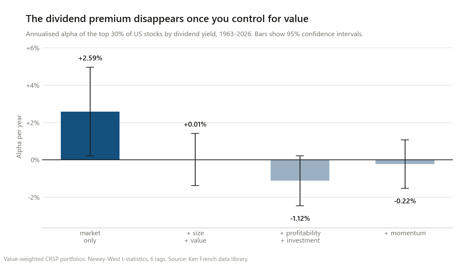
| Model | Alpha/yr | t-stat | Verdict |
|---|---|---|---|
| Market only (CAPM) | +2.59% | 2.14 | Significant |
| + size + value (FF3) | +0.01% | 0.02 | Nothing left |
| + profitability + investment (FF5) | −1.12% | −1.64 | Nothing left |
| + momentum | −0.22% | −0.34 | Nothing left |
Top 30% by dividend yield, 1963–2026, 756 months. Newey-West t-statistics, 6 lags.
Adding two factors moved alpha from a statistically significant +2.59% a year to +0.01%. Not “reduced”. Erased. The 95% confidence interval on that second bar runs from about −1.4% to +1.4% — a range in which zero is the single most likely value.
The cleaner version of the test is a long-short portfolio: buy the top 30% by yield, short the bottom 30%, which isolates the dividend tilt and cancels out most of the market.
| High-minus-low dividend spread | Alpha/yr | t-stat |
|---|---|---|
| Raw return difference | +0.92pp | — |
| Market only | +2.77% | 1.79 |
| + size + value | −0.61% | −0.55 |
| + profitability + investment | −1.09% | −0.95 |
| + momentum | +0.14% | 0.12 |
Not one of these is statistically distinguishable from zero once value is included.
What these portfolios are actually made of
The factor loadings say plainly what the sort is doing:
| Portfolio | Market | Size | Value | Profitability | Investment |
|---|---|---|---|---|---|
| Top 30% dividend yield | 0.87 | −0.03 | +0.48 | +0.20 | +0.20 |
| Middle 40% | 1.00 | −0.06 | +0.11 | +0.30 | +0.27 |
| Bottom 30% | 1.09 | −0.03 | −0.13 | +0.23 | −0.08 |
| Pays no dividend | 1.13 | +0.52 | −0.24 | −0.18 | −0.37 |
The high-yield portfolio carries a +0.48 loading on value and a below-market beta of 0.87. The long-short spread loads +0.62 on value — that single number is most of the story. Buying high-dividend stocks is, in factor terms, roughly two-thirds of a value bet with a side of low beta.
The bottom row is worth its own moment. Non-dividend-payers are small, expensive, unprofitable, and aggressive investors of capital — the classic junk profile — with 28% volatility and a −90.3% worst drawdown. This is why “dividend payers beat non-payers” is such a misleading framing. You are not comparing dividends to no dividends. You are comparing profitable value companies to speculative unprofitable ones.
Where the answer flips
Averaging over a century hides that this varies enormously by decade:
| Period | High yield | Low yield | Spread | Non-payers |
|---|---|---|---|---|
| 1927–1959 | 9.78% | 9.30% | +0.49pp | 8.91% |
| 1960s–70s | 9.93% | 6.63% | +3.30pp | 6.96% |
| 1980–1999 | 16.87% | 16.72% | +0.15pp | 15.85% |
| 2000s | 5.46% | −0.81% | +6.27pp | −3.39% |
| 2010s | 12.48% | 11.69% | +0.80pp | 14.90% |
| 2020–2026 | 14.29% | 20.96% | −6.67pp | 13.97% |
The dividend tilt’s two great decades were the 1970s and the 2000s — both periods when value beat growth decisively. Its worst stretch is the one we are living in: since 2020, high-yield stocks have trailed low-yield stocks by 6.67 percentage points a year.
That pattern is not a coincidence, and it is the thesis restated in a different form: the dividend strategy wins exactly when value wins, because it substantially is value.
So is dividend investing bad?
No, and I want to be careful here, because “there is no alpha” is not the same claim as “this is a bad idea”.
What the data does not support: that dividends themselves generate excess return, or that a dividend screen is a way to beat the market. There is no evidence of that in ninety-nine years of US data once you control for what the screen is actually selecting.
What the data is consistent with: a high-dividend portfolio being a perfectly reasonable way to hold a value-and-quality tilt with lower-than-market beta (0.87). If that is what you want, this delivers it.
The honest framing is that a dividend screen is a crude value screen with a behavioural benefit — it is much easier to hold through a crash when cash keeps arriving. That benefit is real and it is not in any regression. But you should know that is what you are buying, because there are more direct ways to buy a value tilt, and they do not carry the tax drag of forced income.
That last point matters more than the alpha question for most people, and I have since measured it: the tax on a high-yield fund’s dividends costs about 0.79 points a year at the top qualified rate — roughly eighty times the premium computed above. There is also the question of whether a dividend growth screen does better than a yield screen, which I tested separately: it did, by 0.78 points a year, and the difference turned out to be one factor.
Consistent with the pattern in the market-timing work here — the best days cluster inside drawdowns, perfect timing is worth about 10–14% — the effects people argue hardest about tend to be smaller than claimed, and made of something other than what the name suggests.
Method notes and limitations
- These are Ken French’s portfolios, not mine. Value-weighted CRSP universe, sorted on D/P at the end of each June, rebalanced annually. Using his construction rather than rolling my own removes a large degree of freedom that would otherwise let me tune the answer.
- The sample is held fixed in the headline test. FF5 cannot be built before July 1963 because RMW and CMA do not exist earlier, so a naive comparison of CAPM (1927–) against FF5 (1963–) confounds the model change with a period change. Every alpha in the chart and the main table runs on the identical 1963–2026 window. The full-sample numbers are in the script and tell the same story: FF3 alpha of +0.16%, t = 0.22.
- Newey-West standard errors, 6 lags, since monthly factor residuals are autocorrelated and plain OLS t-stats would overstate significance.
- Absence of alpha is not proof of absence. These are wide confidence intervals. What I can say is that the data does not support a dividend premium, not that one is impossible.
- No taxes, costs, or turnover. This matters more than usual here: dividends are taxed as they arrive, in the year they arrive, whether or not you want the income. A real taxable investor’s result would be worse than shown, and worse than the low-yield portfolio’s.
- Factor models are a lens, not the truth. HML is one particular definition of value. A different definition would move these numbers somewhat, though a +0.48 loading is far too large to be a definitional artefact.
- US only, and dividend policy is not universal. Payout norms differ by country and have shifted over time as buybacks replaced dividends. I would not port this conclusion to another market without rerunning it.
This is research, not personalised financial advice.
The code
def regress(y, X):
    """OLS with Newey-West (HAC) standard errors. Returns annualised alpha."""
    d = pd.concat([y, X], axis=1).dropna()
    res = sm.OLS(d.iloc[:, 0], sm.add_constant(d.iloc[:, 1:])).fit(
        cov_type="HAC", cov_kwds={"maxlags": 6})
    return {"alpha": res.params["const"] * 12, "t": res.tvalues["const"]}


# the whole argument in four lines
excess = dp["Hi 30"] - rf
for name, factors in [("CAPM", CAPM), ("FF3", FF3), ("FF5", FF5), ("FF5+MOM", FF6)]:
    r = regress(excess, factors.reindex(excess.index))
    print(name, f"alpha {r['alpha']:+.2%}/yr  t={r['t']:.2f}")
All data is from the Ken French data library: portfolios formed on D/P, the three- and five-factor series, and the momentum factor.
If you re-run it and get something different, I want to know.